Step 5: Design for Transport Lag7 min read
The distance between the web tangent-point departure from the stock roll and the edge guide sensor is roughly 1m. The operational range of 100 feet-per-minute (fpm) to 2000 fpm converts as 0.5 m/s to 10m/s web speed range.
With a 1-meter sensor distance, the lag at a low speed of 100 fpm (0.5m/s) is 2 seconds. At 2000 fpm (10 m/s) it’s 0.1 second. There will be many tenths transport time delay in production operation.
A transport lag model leads to a gain scaling method to produce a robust linear controller over the range of production web speeds. The figure below illustrates the phase fall-off we can expect from delay time to Edge Guide sensor output over the range of operating web speed.
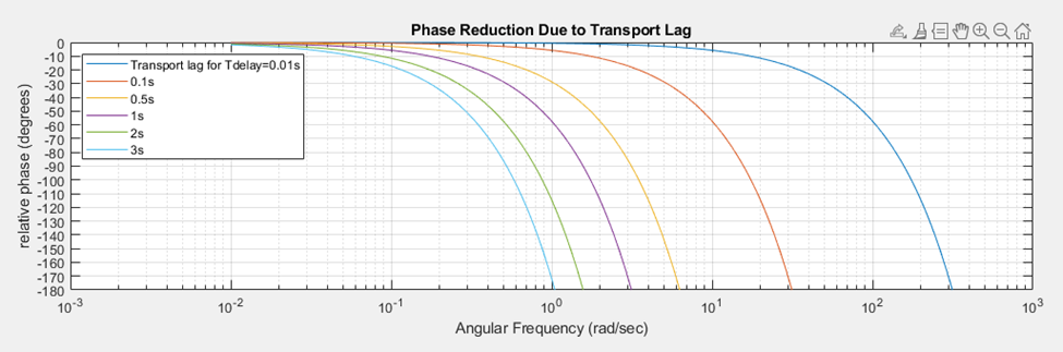
Table of Contents
Compensator Design
Assume a compensator integrator as a design start. We need to integrate out paper edge sensor saturation and account for expected steady-state error even though the plant exhibits and integrating pole.
The edge sensor has a small linear region near the zero-output or on-track regulation point. Off to one side outputs 0 to +10 volts for 6mm or so until saturating at +10V. Off the other way outputs similarly to -10V. If the paper edge is well past the output saturation point a proportional gain alone can not be guaranteed to pull the edge into the sensor’s linear region. Therefore, assume the integrator for the outer loop to account for this large-error saturation region.
We also expect that the integrating plant pole alone, while on paper sufficient to drive to zero steady-state position error, will not do so in practice. The outer-loop integrator will account for bias errors also.
Compensator and Plant System Block Diagram
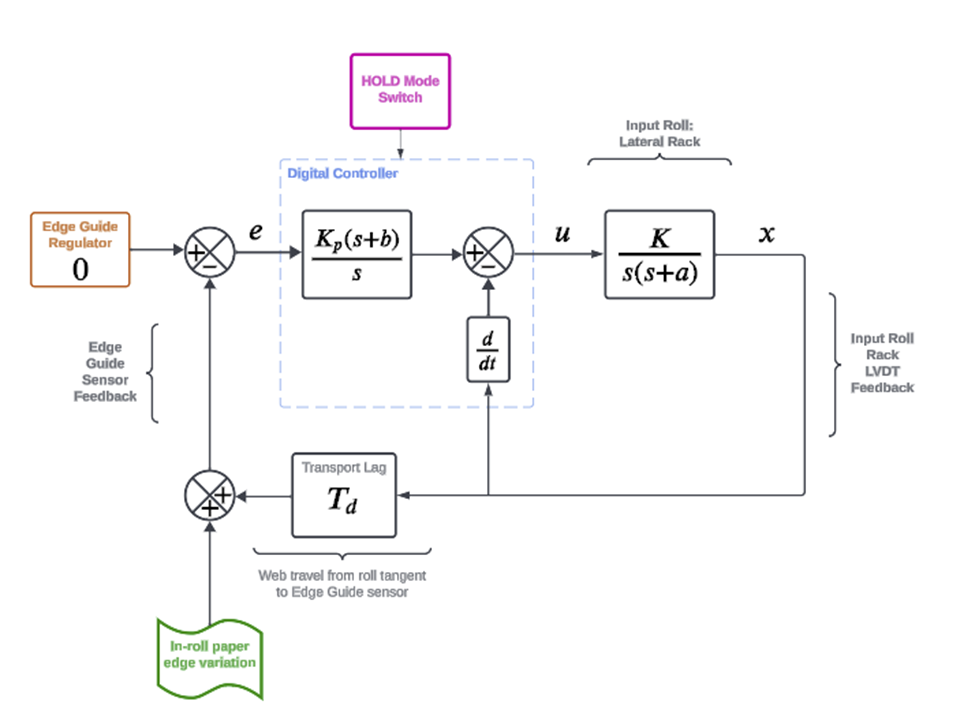
Assuming an integrating pole in our compensator, to achieve sufficient phase margin required for accommodating transport lag at unity-gain crossover as described previously we need to cancel the compensator pole with a zero considerably lower in frequency than the plant bandwidth (the second plant pole at ‘a’). This will produce a wide phase hump that transport lag will then reduce. Represent this compensator zero as, ‘b’ and arrive at a block diagram below. The figure below assumes unity gain for the inner loop driving valve command voltage u.
Ignore the “hold mode” for now. This will be described later as a simple proportional, inner-loop-only mode to simply “hold” rack position according to LVDT feedback during reload and set up when there is no web of paper within the ultrasonic edge sensor.
Compensator Zero Location
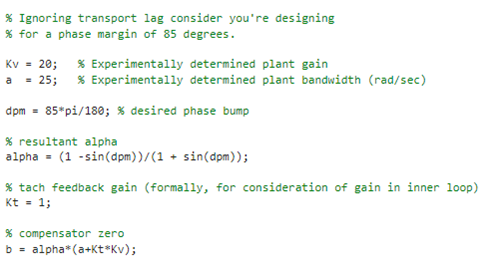
System identification yields the gain ‘Kv’ and pole ‘a’ plant parameters in the Matlab code snippet below. Desiring maximum possible accommodation for transport lag drives a desire for maximum possible phase peak knowing transport lag will reduce the large phase advance. This maximum phase hump is taken at 85 degrees. Lead ratio alpha is calculated as the scalar on plant pole ‘a’ to arrive at controller zero ‘b’.
Controller Gain Plan
With plant pole ‘a’ at 25 rad/sec with a plant pole and a compensator pole we know unity gain crossover design point must be a fraction of 25 radians per second.
A unity gain open-loop crossover frequency of wmax=10 rad/sec is selected. At this design point we compute a corresponding controller gain Kpmax. Given controller zero location ‘b’ this produces a slow responding design with phase margin near 80-degrees at crossover.
However, likely minimum transport delay will be 0.1 seconds for very high 2000 feet-per-minute operation. The system will typically operate with many tenths web transport delay which will diminish the design-point performance that assumes zero transport lag.
The controller will vary gain Kp according to web speed as the measure of transport lag. Hence the controller will be sliding unity-gain crossover as a function of speed. This starting assumption for wmax=10 rad/sec sets the value the controller will scale down from according to web speed.
Web Speed Gain Scaling
the low operational speed range is 100 fpm. This bounds maximum transport time delay at 2 seconds. Maximum operating speed of 2000 fpm gives a minimum transport time delay of 0.1 seconds. By measuring web speed we maintain a real-time estimate of this delay. We assume our design phase hump is nominally 80-degrees and flat over our operating range.
Desiring roughly 50-degrees of phase margin we calculate the angular frequency at which our measured time delay declines to -30 degrees of phase (50=80 minus 30). Pick this as the desired unity-gain crossover frequency relative to wmax and scale Kp down from Kpmax. We leave the lag zero fixed at ‘b’. The fixed zero maximizes the phase lead and you can see in the figure that the range of transport phase lags operate nearest the plant pole ‘a’ and not the lag zero ‘b’. Moving the lag zero won’t buy additional phase lead subject to this range of transport lag. Speeding it slightly for high-speed operation offers offers little value in slight responsive increase ad high web speeds.
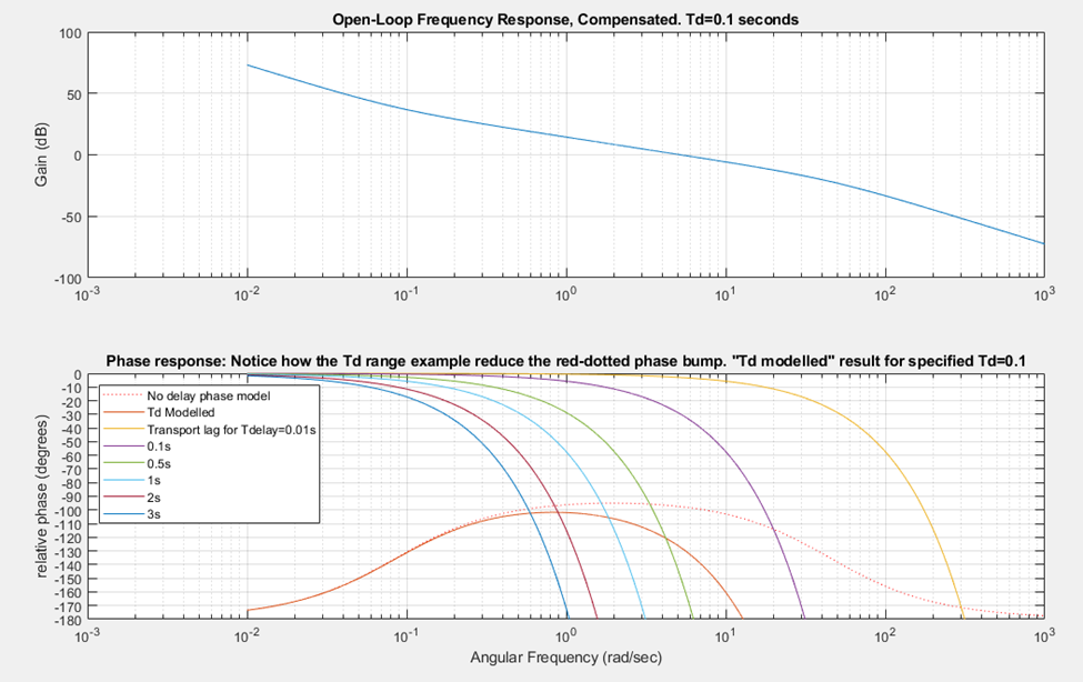
Compensator and Plant Open-Loop Frequency Response
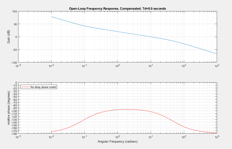
Absent transport lag we would not place compensator zero ‘b’ so low in frequency such that the dotted-orange phase advance would yield over 80-degrees of phase margin. We would place the zero at a higher frequency for a design phase margin of say 50 degrees.
However, when we overlay the phase decline introduced by transport lag this zero-delay design point phase advance (dotted-orange) reduces to the solid orange as shown in the figure below. A 0.1s transport lag is assumed here. The figure illustrates setting controller gain Kp at the point where this orange phase hump exhibits 50 degrees of phase margin according to the scaling logic described earlier.
The controller zeros proportional gain (Kp) to for measured roll speed below ~70 feet per minute (0.35 m/s). This speed is so low as to produce a near 3-second delay between roll-departure tangent and the edge sensor a meter or-so downstream. You can see from the phase plots that past 3 seconds delay transport lag dominates any phase advance offered by the compensator zero. This is adequate as no such low speed is employed for production operations. Slow setup speed and alignment is managed via a second mode entered via a pendant switch: “Hold-Jog” mode.
A Walk-Through Explanation
The control scheme described above is described here with reference to system components. The production form factor PLC pointed to in the box is described in a later post.
Next Up: Hold/Jog Mode for Setup and Reload

