Step 3: System Identification
Neglecting for now the ultrasonic Edge Guide sensor we first seek a model from hydraulic servo valve amplifier voltage command input to LVDT output. This will give us a plant model for the input role lateral position rack. The Edge Guide will provide additional state feedback for our eventual controller, subject to transport lag as we will see.
The diagram below indicates the assumed sub-system elements that collapse down to a plant gain and a plant bandwidth represented by a single pole. There is no storage element in the rack setup or spring, just the moving mass and mechanical resistance (friction) in the setup.
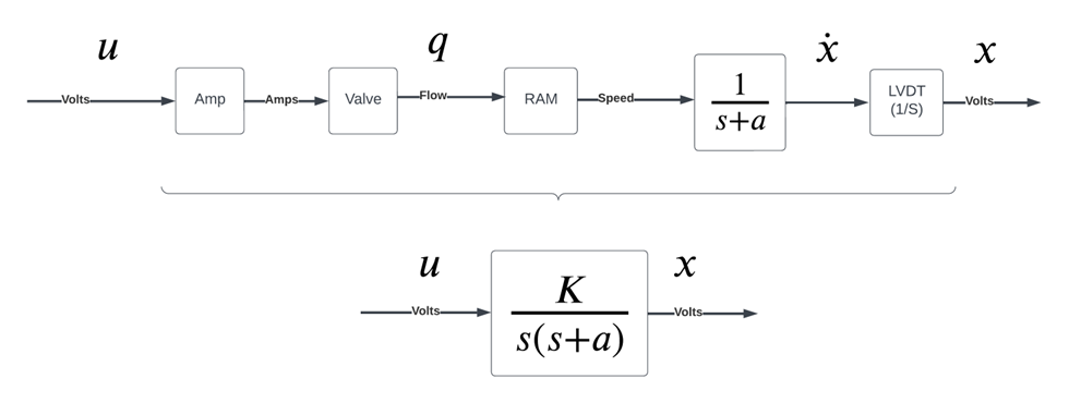
We could likely find the pole ‘a’ by eye with a few sine sweeps. We can use datasheets and estimates to estimate the gain path from amplifier command voltage ‘u’ through to slide rate (xdot). However, for the plant gain in particular we are best suited to perform a sine-sweep system identification and let the data advise us regarding plant gain in particular and with that, pole, ‘a’ also.
Plant Transfer Function Parameter Estimation
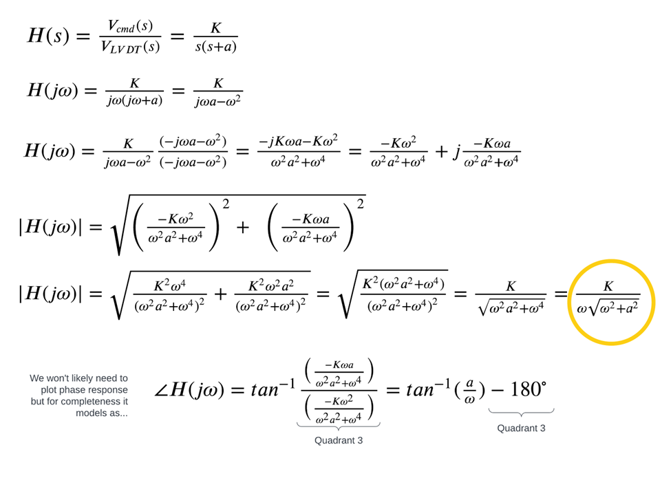
We seek to extract plant gain, ‘K’ and pole location ‘a’ from a log-magnitude plot covering a range of input frequencies and amplitudes. The figure below manipulates our model assumption so we know where to look on our plot to extract plant gain, ‘K’. We discern pole location, ‘a’ from a break frequency revealed by asymptotes sketched over experimental data.
System Identification Procedure
The lateral slide offers roughly 10cm of travel. The maximum command voltage to slew either direction is 5-volts magnitude. A one- or two-volt amplitude sinusoid seems a reasonable signal to sweep over frequency.
The video is a sample of the process for one frequency. Note the system is loaded with a stock roll. Given the apparent mass of the rack system and observation of the dynamics when loaded and unloaded the effect of stock mass variation is taken to be negligible.
System Identification Results
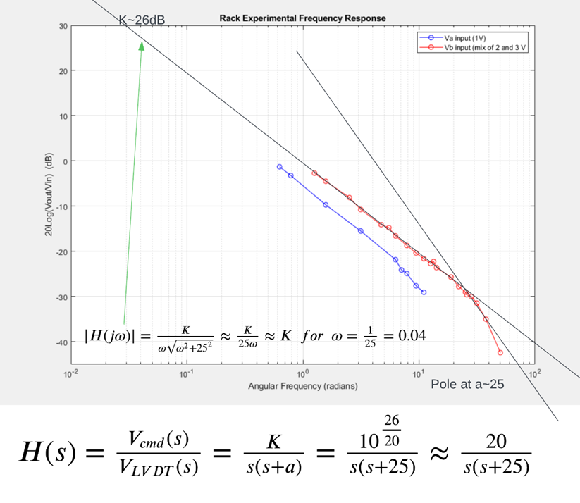
Response to 1-volt input amplitide is plotted in blue below. 2-volt response is shown in red. 3-volts was spot-checked to produce the same results as the 2-volt plot. Between 1 and 2 volts the roughly 6 db (factor of 2) gain difference moves towards the 2-volt result. We will actuate considerably in the small-signal region (deviations of 1 volt and below) but it will be the larger signal response that dictates relative stability.
Therefore we call the 2-volt response large-signal and estimate plant bandwith and gain, ‘K’ from the red plot. The plant will offer less gain for smaller signals as evidenced by the blue samples. Assume our compensator will account for plant gain variation, as is the primary intent of feedback control.
The log-magnitude plot below gives us a plant model transfer function estimate to use in designing a controller.